Erforderliche Pakete laden
library(car)      # MANOVA
library(afex)     # ANOVA
library(heplots)  # HE Plot
library(candisc)  # Diskriminazfunktionsplots
Datensatz einlesen und Variablen spezifizieren
# Datensatz einlesen
Geschlecht <- as.factor(rep(c("männlich","weiblich"), each = 4, times = 3))
Medikament <- as.factor(rep(c("a1","a2","a3"),  each=8))
x1 <- c(5,5,9,7,7,6,9,8,7,7,9,6,10,8,7,6,21,14,17,12,16,14,14,10)
x2 <- c(6,4,9,6,10,6,7,10,6,7,12,8,13,7,6,9,15,11,12,10,12,9,8,5)
data <- data.frame(Geschlecht, Medikament, x1, x2)

# Variablen spezifizieren
Faktoren <- c("Geschlecht", "Medikament")   # Namen der Faktoren mit unabhängigen Stichproben eingeben
AV <- c("x1", "x2")                         # Namen der abhängigen Variablen eingeben
Deskriptive Statistik, Signifikanztest
# Listwise Deletion (Zeilen mit Missings in den berücksichtigten Variablen eliminieren)
data2 <- na.omit(data[,c(AV, Faktoren)])
# Der Datensatz muss eine Spalte "Block" mit den Probanden-IDs enthalten.
data2$Block <- as.factor(1:nrow(data2))

# Deskriptive Statistik
# Zu berechnende Kennwerte spezifizieren.
Kennwerte <- function(x) c(mean = mean(x), sd = sd(x), se=sd(x)/sqrt(length(x)))
# Tabelle
Formel <- as.formula(paste(".~", paste(Faktoren, collapse="+")))
tab <- aggregate(Formel, data2[,c(Faktoren, AV)], Kennwerte)
n <- aggregate(Formel, data2[,c(Faktoren, AV[1])], length)
deskriptive.statistik <- data.frame(tab,n=n[,ncol(n)])

# MANOVA: Quadratsummenzerlegung nach Modell III
library(car)
RS <- paste("C(", Faktoren[1], ",contr.helmert)", sep="")
if (length(Faktoren)>1){
    for (i in 2:length(Faktoren)) RS <- paste(RS, "*C(", Faktoren[i], ",contr.helmert)", sep="")
}
model <- as.formula(paste("cbind(",paste(AV,collapse=","),")~",RS, sep=""))
fit <- lm(model, data=data2)
man.res <- Manova(fit, type="III")
TAB.MANOVA <- summary(man.res, multivariate=TRUE)

# Effektstärken der MANOVA
library(heplots)
eta.sq <- etasq(man.res)

# ANOVAs: Quadratsummenzerlegung nach Modell III
library(afex)
TAB.ANOVA <- list()
for (i in 1:length(AV)){
  TAB.ANOVA[[i]] <- aov_ez(id="Block", dv=AV[i], data=data2, between=Faktoren, return="Anova")
}
names(TAB.ANOVA) <- AV

list("Deskriptive Statistik" = deskriptive.statistik, MANOVA=TAB.MANOVA, Effektstärke=eta.sq, ANOVAs=TAB.ANOVA)
## $`Deskriptive Statistik`
##   Geschlecht Medikament    x1.mean      x1.sd      x1.se   x2.mean     x2.sd
## 1   männlich         a1  6.5000000  1.9148542  0.9574271  6.250000  2.061553
## 2   weiblich         a1  7.5000000  1.2909944  0.6454972  8.250000  2.061553
## 3   männlich         a2  7.2500000  1.2583057  0.6291529  8.250000  2.629956
## 4   weiblich         a2  7.7500000  1.7078251  0.8539126  8.750000  3.095696
## 5   männlich         a3 16.0000000  3.9157800  1.9578900 12.000000  2.160247
## 6   weiblich         a3 13.5000000  2.5166115  1.2583057  8.500000  2.886751
##       x2.se n
## 1  1.030776 4
## 2  1.030776 4
## 3  1.314978 4
## 4  1.547848 4
## 5  1.080123 4
## 6  1.443376 4
##
## $MANOVA
##
## Type III MANOVA Tests:
##
## Sum of squares and products for error:
##      x1    x2
## x1 94.5  76.5
## x2 76.5 114.0
##
## ------------------------------------------
##
## Term: (Intercept)
##
## Sum of squares and products for the hypothesis:
##        x1       x2
## x1 2281.5 2028.000
## x2 2028.0 1802.667
##
## Multivariate Tests: (Intercept)
##                  Df test stat approx F num Df den Df     Pr(>F)
## Pillai            1  0.960659 207.5601      2     17 1.1381e-12 ***
## Wilks             1  0.039341 207.5601      2     17 1.1381e-12 ***
## Hotelling-Lawley  1 24.418839 207.5601      2     17 1.1381e-12 ***
## Roy               1 24.418839 207.5601      2     17 1.1381e-12 ***
## ---
## Signif. codes:  0 '***' 0.001 '**' 0.01 '*' 0.05 '.' 0.1 ' ' 1
##
## ------------------------------------------
##
## Term: C(Geschlecht, contr.helmert)
##
## Sum of squares and products for the hypothesis:
##           x1        x2
## x1 0.6666667 0.6666667
## x2 0.6666667 0.6666667
##
## Multivariate Tests: C(Geschlecht, contr.helmert)
##                  Df test stat   approx F num Df den Df  Pr(>F)
## Pillai            1 0.0074631 0.06391302      2     17 0.93831
## Wilks             1 0.9925369 0.06391302      2     17 0.93831
## Hotelling-Lawley  1 0.0075192 0.06391302      2     17 0.93831
## Roy               1 0.0075192 0.06391302      2     17 0.93831
##
## ------------------------------------------
##
## Term: C(Medikament, contr.helmert)
##
## Sum of squares and products for the hypothesis:
##       x1       x2
## x1 301.0 97.50000
## x2  97.5 36.33333
##
## Multivariate Tests: C(Medikament, contr.helmert)
##                  Df test stat approx F num Df den Df     Pr(>F)
## Pillai            2  0.880378  7.07686      4     36 0.00026018 ***
## Wilks             2  0.168630 12.19913      4     34 2.9586e-06 ***
## Hotelling-Lawley  2  4.639537 18.55815      4     32 5.5968e-08 ***
## Roy               2  4.576027 41.18424      2     18 1.9190e-07 ***
## ---
## Signif. codes:  0 '***' 0.001 '**' 0.01 '*' 0.05 '.' 0.1 ' ' 1
##
## ------------------------------------------
##
## Term: C(Geschlecht, contr.helmert):C(Medikament, contr.helmert)
##
## Sum of squares and products for the hypothesis:
##          x1       x2
## x1 14.33333 21.33333
## x2 21.33333 32.33333
##
## Multivariate Tests: C(Geschlecht, contr.helmert):C(Medikament, contr.helmert)
##                  Df test stat approx F num Df den Df  Pr(>F)
## Pillai            2 0.2269491 1.151992      4     36 0.34808
## Wilks             2 0.7743623 1.159326      4     34 0.34590
## Hotelling-Lawley  2 0.2896916 1.158766      4     32 0.34728
## Roy               2 0.2837227 2.553504      2     18 0.10562
##
## $Effektstärke
##                                                                 eta^2
## (Intercept)                                               0.960659099
## C(Geschlecht, contr.helmert)                              0.007463063
## C(Medikament, contr.helmert)                              0.440189051
## C(Geschlecht, contr.helmert):C(Medikament, contr.helmert) 0.113474526
##
## $ANOVAs
## $ANOVAs$x1
## Anova Table (Type III tests)
##
## Response: dv
##                        Sum Sq Df  F value    Pr(>F)
## (Intercept)           2281.50  1 434.5714 4.704e-14 ***
## Geschlecht               0.67  1   0.1270    0.7257
## Medikament             301.00  2  28.6667 2.538e-06 ***
## Geschlecht:Medikament   14.33  2   1.3651    0.2806
## Residuals               94.50 18
## ---
## Signif. codes:  0 '***' 0.001 '**' 0.01 '*' 0.05 '.' 0.1 ' ' 1
##
## $ANOVAs$x2
## Anova Table (Type III tests)
##
## Response: dv
##                        Sum Sq Df  F value    Pr(>F)
## (Intercept)           1802.67  1 284.6316 1.776e-12 ***
## Geschlecht               0.67  1   0.1053   0.74934
## Medikament              36.33  2   2.8684   0.08292 .
## Geschlecht:Medikament   32.33  2   2.5526   0.10569
## Residuals              114.00 18
## ---
## Signif. codes:  0 '***' 0.001 '**' 0.01 '*' 0.05 '.' 0.1 ' ' 1
Grafiken
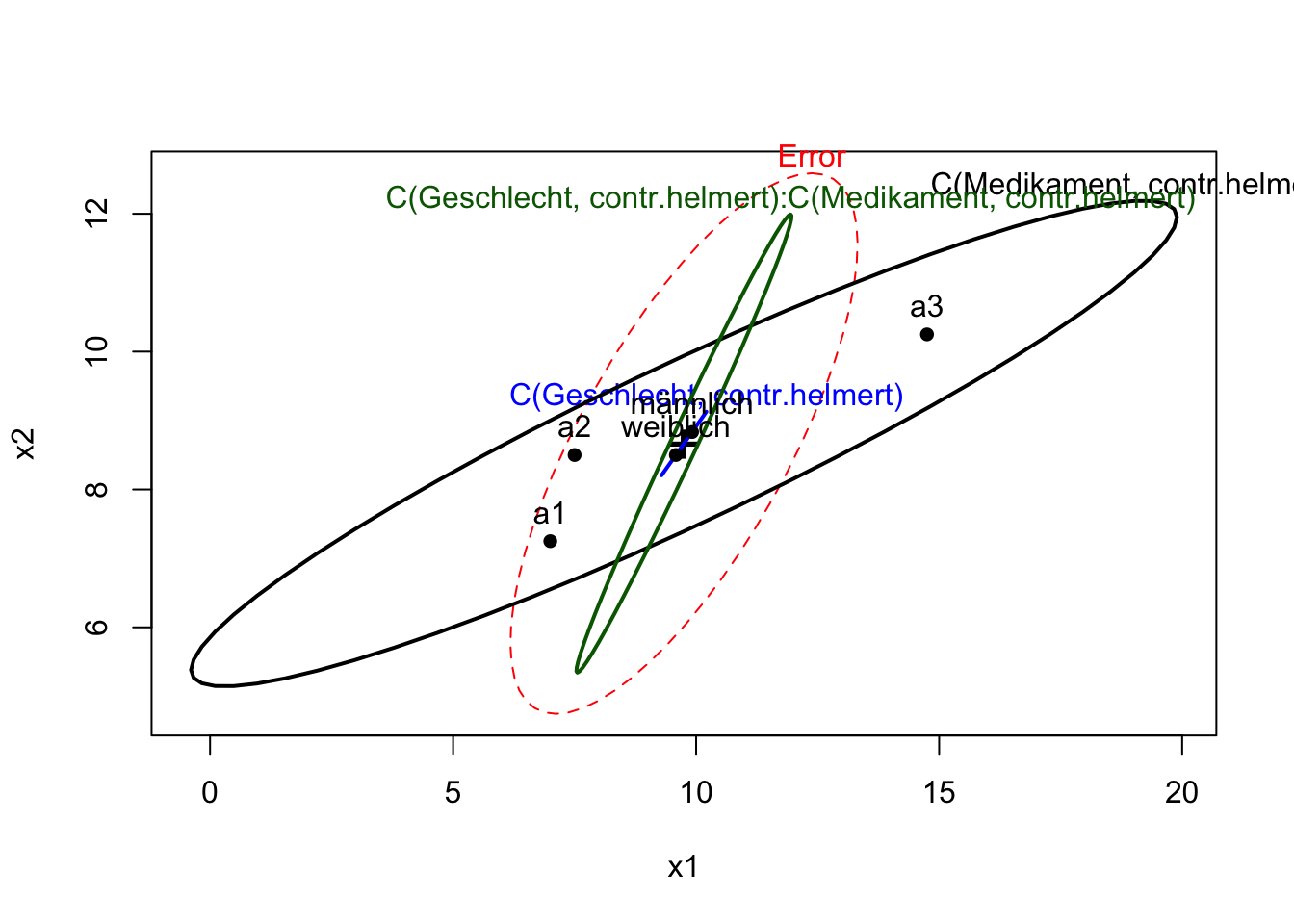
# HE-Plots
if (length(AV)==2){
  heplot(fit)
} else{
  pairs(fit)
}
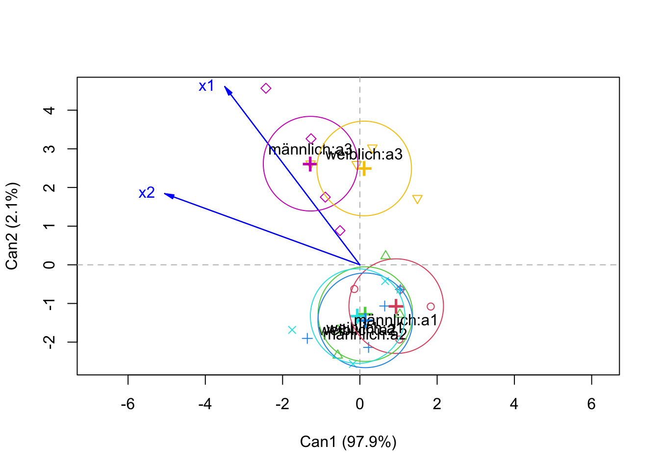
# Diskriminazfunktionsplots
library(candisc)
term <- "Geschlecht:Medikament"
model <- as.formula(paste("cbind(",paste(AV,collapse=","),")~",paste(Faktoren,collapse="*"),sep=""))
fit2 <- lm(model, data=data2)
can <- candisc(fit2, term=term)
plot(can)